The importance of knowing your data“Data, data, data! I cannot make bricks without clay!” Good old Sherlock, a quote for every occasion… ("The Adventure of the Copper Beeches" Sir Arthur Conan Doyle, 1892) We in the 21st Century have access to a huge volume of data. More than any generation before us. And with each day that volume of data grows ever larger. One of the many consequences of the COVID-19 pandemic has been the continuous news coverage stressing the importance of data. We are regaled daily with graphs and statistics that I imagine few people understand or want to understand. The challenge with all data is working out which are worth using and how to best use this. It is about knowing your data. In the age of AI (Artificial Intelligence) and machine learning, there is a temptation to assume that all we need to do is to ‘train’ our software, load in the data, and wait for the answer. “42” instantly comes to mind - for those of you old enough to remember the prescient imagination of Douglas Adams and “The Hitchhikers Guide to the Universe”. There is no question that both AI and machine learning have a huge potential in helping us better understand the world. Computers provide us with the capability to interrogate the vastness of our data libraries and to draw out patterns and conclusions that we would otherwise not have the time to do. The developments in these techniques are impressive. If you are not convinced check out the Google AI site (https://ai.google/). But we need to be careful. Not because AI is not useful, it is. But because there are fundamental issues around data and analytics that we must answer first:
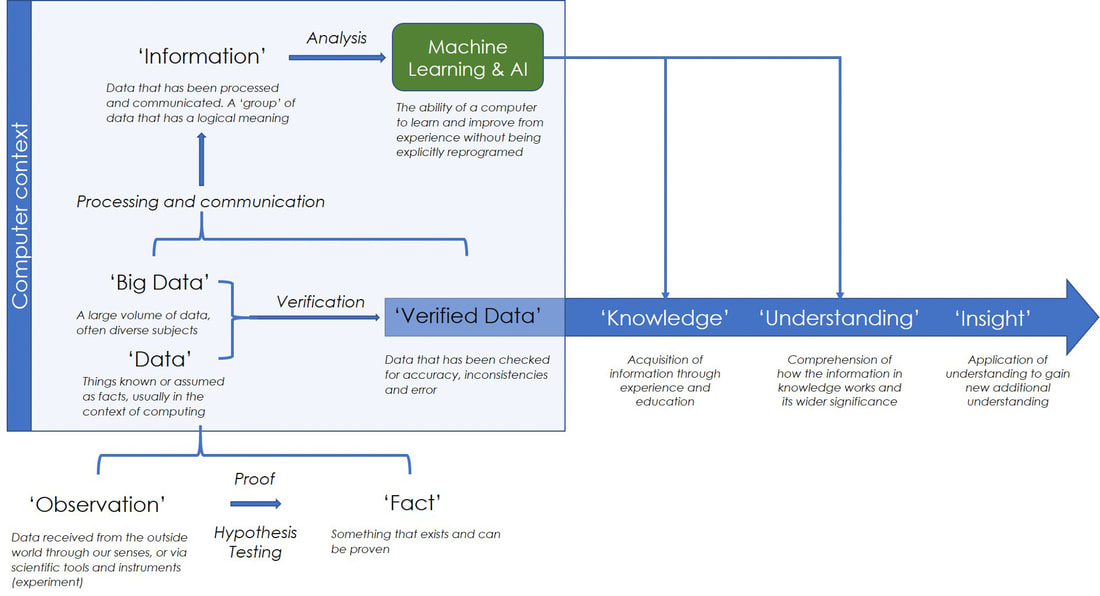
Each merits an essay in its own right. Here, I am going to focus on the third – do we trust our data? Figure 1. We in the 21st Century have access to a huge volume of data. In the last 40 years, we have seen the transition of that data from physical libraries, as illustrated here by a suite of bound scientific papers in my library, to the “1s” and “0s” of the digital age Data, data, data I have spent much of my career designing, building, populating, managing, and analyzing ‘big data’. From using paleobiological observations to investigate global extinction and biodiversity, to testing climate model experiments, to paleogeography, and petroleum and minerals exploration. Having worked at each stage from data collection to data analytics I have gained a unique insight into data, especially big data. Most databases are built to address specific problems, and no surprise, these rarely give us insights beyond the questions originally asked. But when we think of Big Data and AI we are usually thinking of large, diverse datasets with which to explore, to look for patterns and relationships we did not anticipate. My interest has always been in building these sorts of large, diverse ‘exploratory’ databases following in the footsteps of some great mentors I was privileged to have at The University of Chicago, the late Jack Sepkoski, and my Ph.D. advisor Fred Ziegler. ‘Exploratory’ databases have their own inherent challenges, not least the need to ensure that they include information that can address questions that the author has not yet thought of… That is a major problem. This requires specific design considerations, especially, as I argue you here, the fundamental importance of ensuring that we know the source and quality of the data we are using. Because it is upon these data that we base our interpretations, and from those interpretations the understanding and insights we derive. If the data are flawed then everything we do with that data is similarly flawed and we have wasted our time. This is even more important when we are analyzing 3rd party databases that we have not built ourselves. How far can we, should we trust them? In short, we can have the best AI system in the world and the most powerful computers, but if the data we feed the system is rubbish, then all we will get out is rubbish. What do we mean by data? In discussing data and databases it has become de rigueur to quote Conan Doyle: “Data, data, data! I cannot make bricks without clay!” Good old Sherlock, a quote for every occasion… ("The Adventure of the Copper Beeches" Sir Arthur Conan Doyle, 1892) But what do we mean by “data”? When I started to write this article, I thought I knew. But in looking through the literature I soon realized that such terms as “data”, “Big data” and “information” were vaguely defined and used interchangeably. So, to help anyone else in the same position here is a quick look at the terminology, including some that you may or may not be familiar with. This is summarised in figure 1. A more comprehensive set of definitions is provided as supplementary data in the pdf version of this blog article. Figure 2. The relationship between data, information, knowledge, understanding, and insight. This summary figure shows the problem of current definitions (see supplementary data for further information) The fundamental progression here is from data to verified data to knowledge, understanding, and insight (see the recent Linkedin article by the branding company LittleBigFish). Admittedly, in many ways trying to define the relationships between observations, facts, data and information is semantics. For databasing we can reduce this to data and verified data, and this takes us back to the need to audit and qualify our data: the data to verified data transition. The audit trail: Recording Data Provenance and Explanation When designing and building a database we need to ensure that we include information about the data. For spatial geological data, we need to answer a range of questions about the data, including the following:
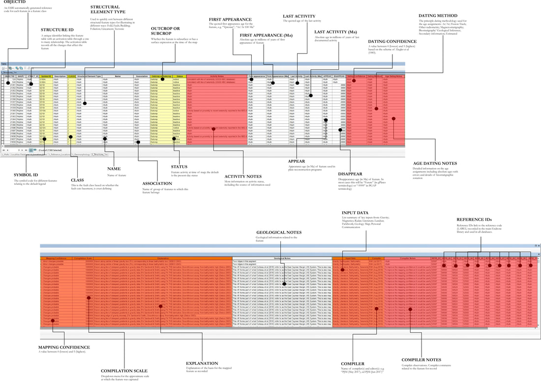
(For further information on this see Markwick & Lupia (2002) Providing the answers to these questions will enable anyone using the database to replicate what was done and to make decisions on how they use the data. Where this applies to the database as a whole it will be recorded within the metadata. The metadata also provides information on the intrinsic characteristics of the data in a database, such as data type, field size, date created, etc. This is different from extrinsic information, such as the input data used for a specific database record. This extrinsic, record specific information is stored within the data tables themselves. For example, in our Structural Elements Database (see figure 3 attribute table), features may be based on an interpretation of one of several primary datasets, including Landsat imagery, radar data, gravity, magnetics, and seismic. This needs to be recorded because each primary dataset will have its inherent resolution and errors. I have always believed that more explanation is required. So, within my own commercial and research databases, I have added text fields for each major inputs to describe the basis of each interpretation. For example, an “Explanation” field provides a place for describing exactly how a spatial feature was defined. All records are then linked to a reference library through unique identifiers (Markwick, 1996; Markwick and Lupia, 2002). This is a relatively standard design. (Nb. In my research, I use the Endnote software, which I have used since my Ph.D. days in Chicago in the 1990s and which I can highly recommend https://endnote.com/) Figure 3. The main attribute table for the Structural Elements database showing in red those fields used to qualify and/or audit each record. Of 38 fields 20 store information that qualifies the entry. In addition, there is the metadata, data documentation, and underlying data management system and workflows. The problem for database design is knowing what level of auditing is needed to adequately qualify an individual record. This will depend on whether the record is of a primary observation – analytical, field measurement, etc – or an interpretation. Interpretations can change with time. For example, a biostratigraphic zonation used 30 years ago may not be valid today, but the primary observations of which organisms are present may still be true (accepting that taxonomic assignments may also change). So in a database of this information, you would need to record not just the zonation (interpretation), but also what it was based on – this might either be a complete list of the organisms present (the approach I took with my Ph.D. databases) or simply a link to the reference which contains that information. Another example that has driven me to frustration over the years is the use of biomarkers in organic geochemistry. Interpretations of these have changed frequently over the last 40 years. For example, the significance of gammacerane (the gammacerane index) which I remember in the 1980s as an indicator of salinity (Philp and Lewis, 1987), but which may (also) indicate water stratification (Damsté et al., 1995), or water stratification resulting from hypersalinity (Peters, Walters and Moldowan, 2007), or none of the above. In both of these examples, we have an analytic error – misidentification of a species down a microscope or errors associated with gas chromography (GC), or GC-mass spectrometry (MS), etc – and an error or uncertainty in the interpretation. In any database, we, therefore, need first to ensure that we differentiate between the two: observation and interpretation. We then need to record auditing information that covers both: what the biomarker is (observation); the analytic error in the observation; the interpretation; a reference to who made the interpretation, when, and why. To which we can add a comments field and a semi-quantitative confidence assignment by the person entering the data into the database (see below). By recording the reference of the interpretation and analysis we can then either parse the data to include or reject it for specific tasks or update the interpretation with the latest ideas. Again, this would be attributed as an update or edit in the database and audited accordingly (in my databases I have a “Compiler” field that lists the initials of the editor and month and year when they made any changes – in corporate databases you may need to have more detail than this). We need to keep track of all these things in a database if the database is to have longevity and application. This is not easy. The consequence is that within a database we end up with most of the fields being about auditing our data, rather than values or interpretation (Figure 3). Scale, Resolution, Grain, and Extent in Digital Spatial Databases In spatial databases we also need to understand scale and resolution. We all ‘know’ what we mean by “map scale”. It is something that is always explicitly stated on a printed, paper map and provides an indication of the level of accuracy and precision we can expect (not always true but our working assumption). But digital maps are a problem. Why? To answer that, ask yourself a simple question “what is the map scale of a digital map?” To understand this question, open up a map image on your laptop or phone and then zoom in. Is the scale the same before and after you zoom? – measure the distance on the screen! The answer is of course “No”. The map image may have a scale written on it, but on the screen, you can zoom in and out as far as you want (Figure 4). This immediately creates a problem of precision and accuracy (see below). How far can we zoom into a digital map before we go beyond the precision and accuracy that the cartographer intended? In building digital spatial databases we can address this in one of several ways
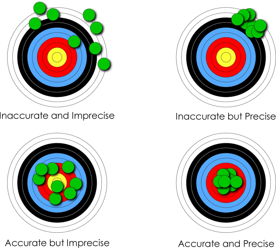
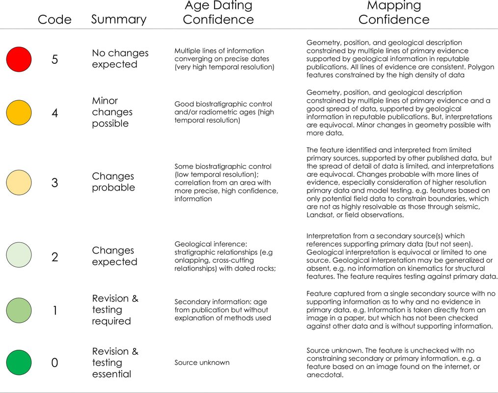
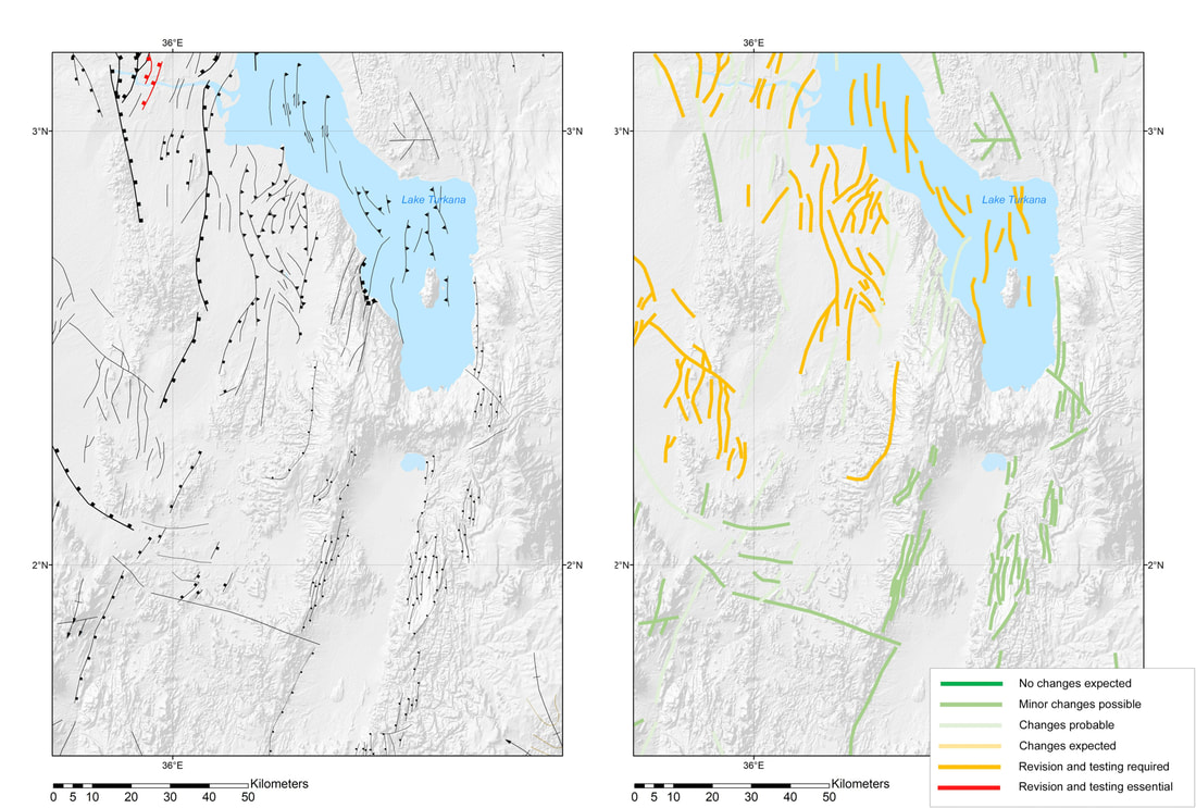
As with all data issues, the importance is being aware there is a potential problem here. Two further terms you may find of use when thinking of spatial data are “grain” and “extent”. These are both adopted from landscape ecology. Grain refers to the minimum resolution of observation, for example, its spatial or temporal resolution (Markwick and Lupia, 2002). Extent is the total amount of space or time observed, usually defined as the maximum size of the study area (O'Neill and King, 1998). So, a large scale map may be fine-grained but of limited extent. The key is specifying this for each study. Figure 4. The same 1:25,000 scale map shown on two different devices but at two different ‘scales’. The tablet shows a zoomed in view – the arrows show the same transect in each case. In neither case are they are 1:25,000. Map source; 1:25,000 topographic maps of Catalonia – this an excellent resource available online Precision and Accuracy Differentiating between precision and accuracy is something of a cliché (see Figure 5). But no less important. A geological observation has a definite location, although it is not always possible to know this with precision, either because the details are/were not reported, or the location was not well constrained originally. Today, with GPS (Global Positioning Systems), problems with location have been mitigated, but not eliminated. For point data, this can be constrained in a database by an attribute that provides an indication of spatial precision. In my databases, this is a field called “Geographic Precision” (Table 1). The precision of lines and polygons can be attributed in a similar way, although in our databases we have used a qualitative mapping confidence attribute which implicitly includes feature precision and accuracy (see below). Temporal precision and accuracy are more difficult to constrain in geological datasets. Ages can be made incorrectly, be based on poorly constrained fossil data, or radiometric data with large error bars. In some cases, there may be no direct age information at all, and the temporal position is based on geological inference. Ziegler et al (1985) qualified age assignments based on their provenance, which we have also adopted. Figure 5. A graphical representation of the difference between accuracy and precision. This is something of a cliché but important to understand nonetheless Table 1 - Geographic precision. This is a simple numerical code that relates the precision with which a point location is known on a map. This allows poorly resolved data to be added to the database when no other data is available, which can be replaced when better location information is known (Markwick, 1996; Markwick and Lupia, 2002). Well data should always be of the highest precision, and indeed should be known within meters Qualifying and quantifying confidence and uncertainty Whilst analytical error is numeric, and sometimes we can assign quantitative values to position or time (± kilometers, meters, millions of years) this is not always possible. So another way to approach the challenge of recording confidence or uncertainty is to have the compiler assign a qualitative or semi-quantitative assessment. In our databases, we again follow some of the ideas outlined in Ziegler et al., (1985), Markwick and Lupia (2001), Markwick (1996). These schemes are distinct from quoted analytical errors and are designed to give the user an easy-to-use ‘indication’ of uncertainty (Table 2). Table 2. Explanation of confidence codes used for structural elements. The age dating confidence is based on the scheme described in Ziegler et al (1985) The advantage of this approach is that it is simple, which encourages adoption. The disadvantage is that even with explanations of what each code represents (Table 2), there will be some user variation. Nonetheless, it provides an immediate indication of what the compiler believes, which can then be further explained in associated comments fields. In map view, colors can be applied to give the users an immediate visualization of mapping or dating or other confidence depending on what the user needs to know. An example of the mapping confidence applied to structural elements is shown in figure 6. Confidence is further expressed visually using shading, dashed symbology, and line weighting (this is discussed in our database documentation and will be the focus of an article I am writing on drawing maps). Figure 6 - A detailed view of the eastern branch of the East African Rift System in the neighborhood of Lake Turkana showing the structural elements from our global Structural Elements database (left) colored according to the assigned mapping confidence (right). The lower confidence assigned to features in the South Sudanese Cretaceous basins (just outside this extent) reflects the use of published maps as the source to constrain features. Although these interpretations may be quoted as based on seismic, as they are, the lack of supporting primary data relegates the confidence to category 2 or in some cases 1. Those upgraded to category 3, indicated by the light green colors, are supported by interpretations from primary sources, such as gravity or better quality seismic. The category 4 features (medium green) in this view are largely based on Landsat imagery constrained by other sources, such as high-resolution aeromagnetic data and seismicity. This gives the user an immediate indication of mapping confidence, which intentionally errs on the side of caution. Features can be upgraded as more data comes available Do we capture all information? By including fields for record confidence means that the database can be sorted (parsed) for good and bad ‘quality’ data. Why is this important? Why not do this on data entry? You could, for example (and I know researchers who do this) make an a priori decision and remove all data that you believe is poor and not include this in the database. But what if this ‘poor’ datum is the only datum for that area or of that type of data that you have? For example, in a spatial database, we may have a poorly constrained data point for a basin (we know its location to within 100 km, but no better), but no other data. That data point is then important or could be, but is spatially poorly constrained – in this case, a low spatial precision. We need to include this record in our database, because it is all we have. But we need to ensure that the record is audited to reflect the uncertainty in its location. A priori decisions on which data to include in our database based on an initial assessment of data confidence are therefore to be avoided:
Who are the database builders? Given how much information we need to record to qualify our data, it will come as no surprise that data entry compliance is a major difficulty. Database population is very tedious. This can result in errors, or short-cuts being taken, or worse. As an example of what can happen, I had one senior geologist, who will remain nameless, point-blank refuse to attribute his interpretations, stating that GIS and attribution “were beneath him”. After pressure, he acquiesced. But during my QC stage, I found that in a fit of pique he had copied and pasted the same attribution for all records – assigning “Landsat imagery” as the source for submarine features was a bit of a giveaway! All of his work had to be redone, by me as it happened… This case highlights a serious challenge, to get staff to realize the importance of the audit trail and to fill in these fields. From my experience let me suggest four ways you can do this (other than threats):
The solution here is to recognize that technology is there to help you reach answers by removing the most tedious repetitive tasks, and analyzing and managing large datasets. But we must never forget that we still need to know our data. It is a truism that the more remote we get from our data the least likely we are to understand any answers our AI system gives us. We also need to remember that databases are ‘living’ in the sense that you cannot, should not simply populate a database and walk away, but recognize that you need to update and add to your database as more information becomes available. It is about knowing your data There is no question that AI and machine learning have much to offer us in data science. But where I worry a little, or perhaps more than a little, about AI is how it is being perceived in many companies as a black-box solution to the problem of big data. We as users need to have enough knowledge to understand the answers such systems give us, but more importantly, as I hope I have demonstrated here in this brief introduction, we need to ensure that we know where our data has come from and that we trust it. This is not just in the sense of computer verification, but in constraining the nature of the original data itself, how it is recorded, how confident we can be with this recording. This process of qualifying and auditing data is admittedly laborious as my examples of solutions show, but I hope you will have seen how powerful even the simplest schemes can be when used systematically. A pdf version of this blog is available here for download. Postscript As some of the more observant readers will have noticed the sediment in the picture at the beginning of this article is not clay, but sand. As I have emphasized throughout, you need to know your data – be careful what you build from References cited Callegaro, M. & Yang, Y. 2018. 23. The role of surveys in the era of "Big Data". In The Palgrave Handbook of Survey Research eds D. L. Vannette and J. A. Krosnick). pp. 175-91.
Damsté, J. S. S., Kenig, F., Koopmans, M. P., Köster, J., Schouten, S., Hayes, J. M. & Leeuw, J. W. d. 1995. Evidence for gammacerane as an indicator of water column stratification. Geochemica et Cosmochimica Acta 59, 1895-900. Markwick, P. J. 1996. Late Cretaceous to Pleistocene climates: nature of the transition from a 'hot-house' to an 'ice-house' world. In Geophysical Sciences p. 1197. Chicago: The University of Chicago. Markwick, P. J. & Lupia, R. 2002. Palaeontological databases for palaeobiogeography, palaeoecology and biodiversity: a question of scale. In Palaeobiogeography and biodiversity change: a comparison of the Ordovician and Mesozoic-Cenozoic radiations eds J. A. Crame and A. W. Owen). pp. 169-74. London: Geological Society, London. O'Neill, R. V. & King, A. W. 1998. Homage to St. Michael or why are there so many books on scale? In Ecological Scale, Theory and Applications eds D. L. Peterson and V. T. Parker). pp. 3-15. New York: Columbia University Press. Peters, K. E., Walters, C. C. & Moldowan, J. M. 2007. The biomarker guide. Volume 2. Biomarkers and isotopes in petroleum systems and Earth history, 2nd ed.: Cambridge University Press, 704 pp. Philp, R. P. & Lewis, C. A. 1987. Organic geochemistry of biomarkers. Annual Review of Earth and Planetary Sciences 15, 363-95. Samuel, A. 1959. Some Studies in Machine Learning Using the Game of Checkers. IBM Journal of Research and Development 3, 211-29. Ziegler, A. M., Rowley, D. B., Lottes, A. L., Sahagian, D. L., Hulver, M. L. & Gierlowski, T. C. 1985. Paleogeographic interpretation: with an example from the Mid-Cretaceous. Annual Review of Earth and Planetary Sciences 13, 385-425.
0 Comments
Leave a Reply. |
AuthorDr Paul Markwick Archives
November 2023
Categories |
|
Copyright © 2017-2024 Knowing Earth Limited
|
E-mail: [email protected]
|


